Combining near-surface geophysical data with the open-source library pyGIMLi

Florian Wagner

RWTH Aachen University

Alexander Jaron

RWTH Aachen University

Nino Menzel

RWTH Aachen University

2026-09-20

Our plan for today

Time Session Lead
09:00-10:30 1. Introduction F. Wagner
10:30-11:00 Break
11:00-12:30 2. Advanced inversion N. Menzel
12:30-13:30 Lunch
13:30-15:00 3. Joint inversion A. Jaron
15:00-15:30 Break
15:30-17:00 4. Additional topics & assisted data processing

Note

Feel free to ask questions at any time during the workshop. We will also have a Q&A session at the end of each part of the workshop.

Interactive slides available here

QR code linking to the workshop slides at https://gimli-org.github.io/nsg26/

Code & slides here:

https://nsg26.pygimli.org

Survey evaluation

Survey evaluation

Introduction

Geophysical monitoring of subsurface processes
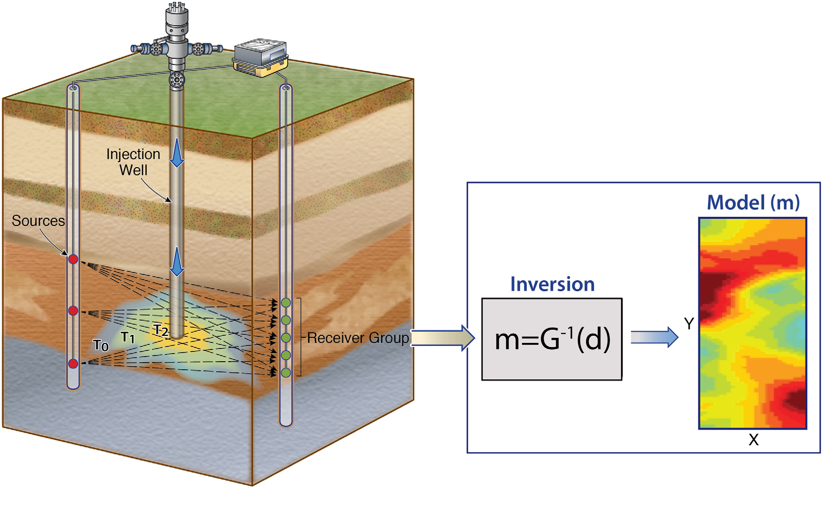
Binley et al. (2015)

Quantitative imaging and monitoring is challenging
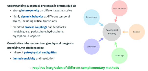
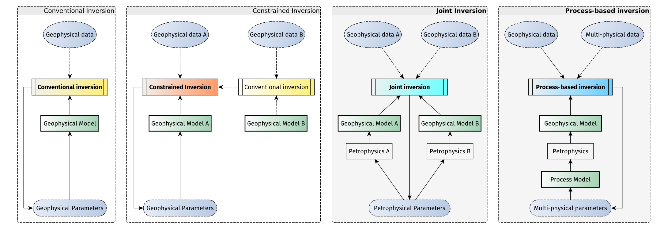
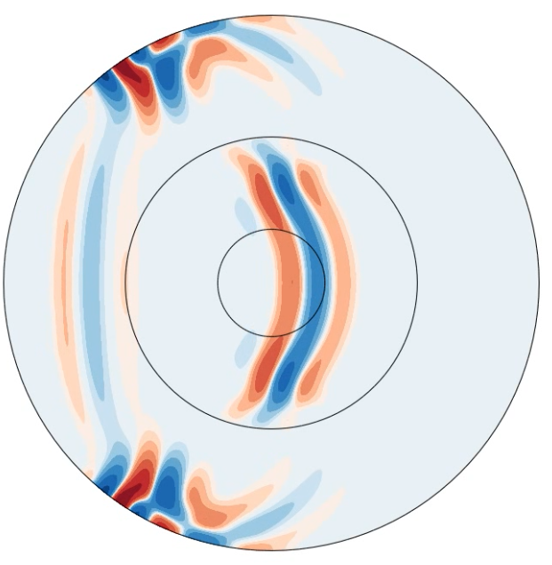
The evolution of geophysical imaging for subsurface characterization
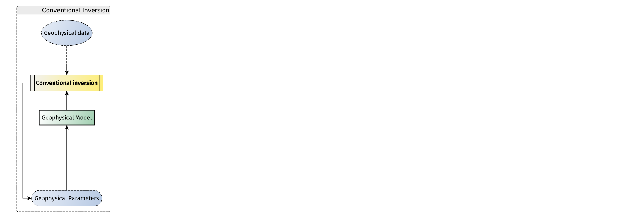
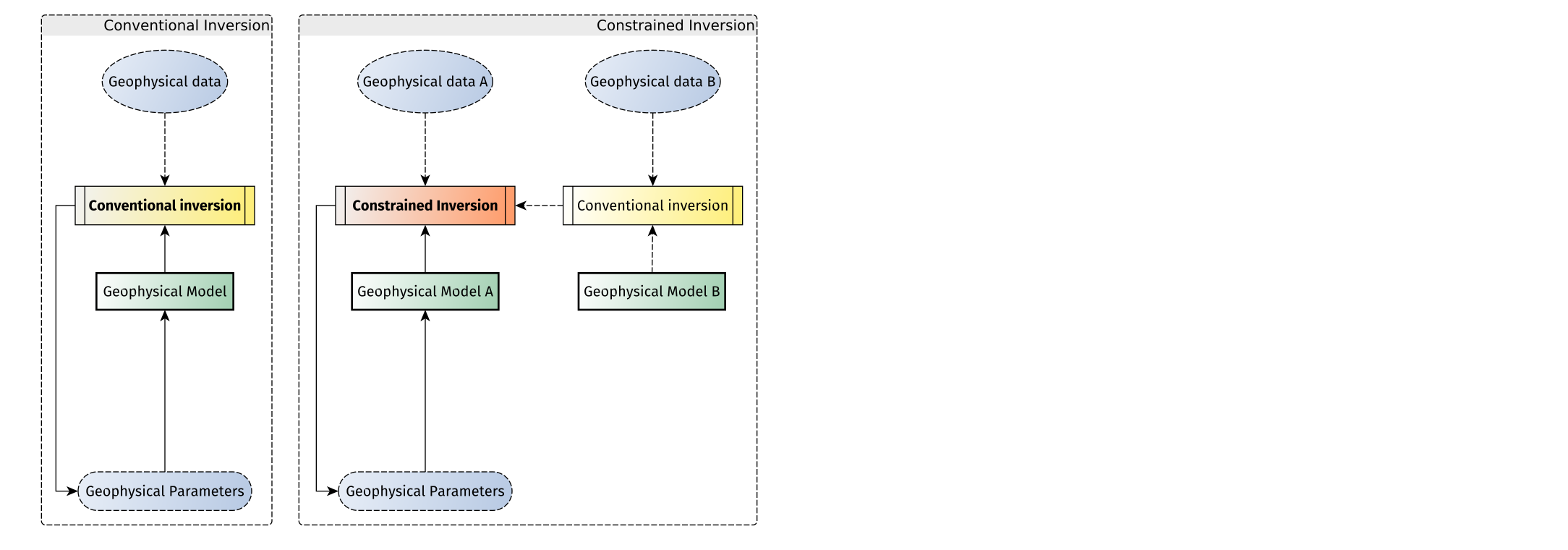
(Wagner & Uhlemann, 2021)

–> model coupling is challenging and requires versatile open-source software

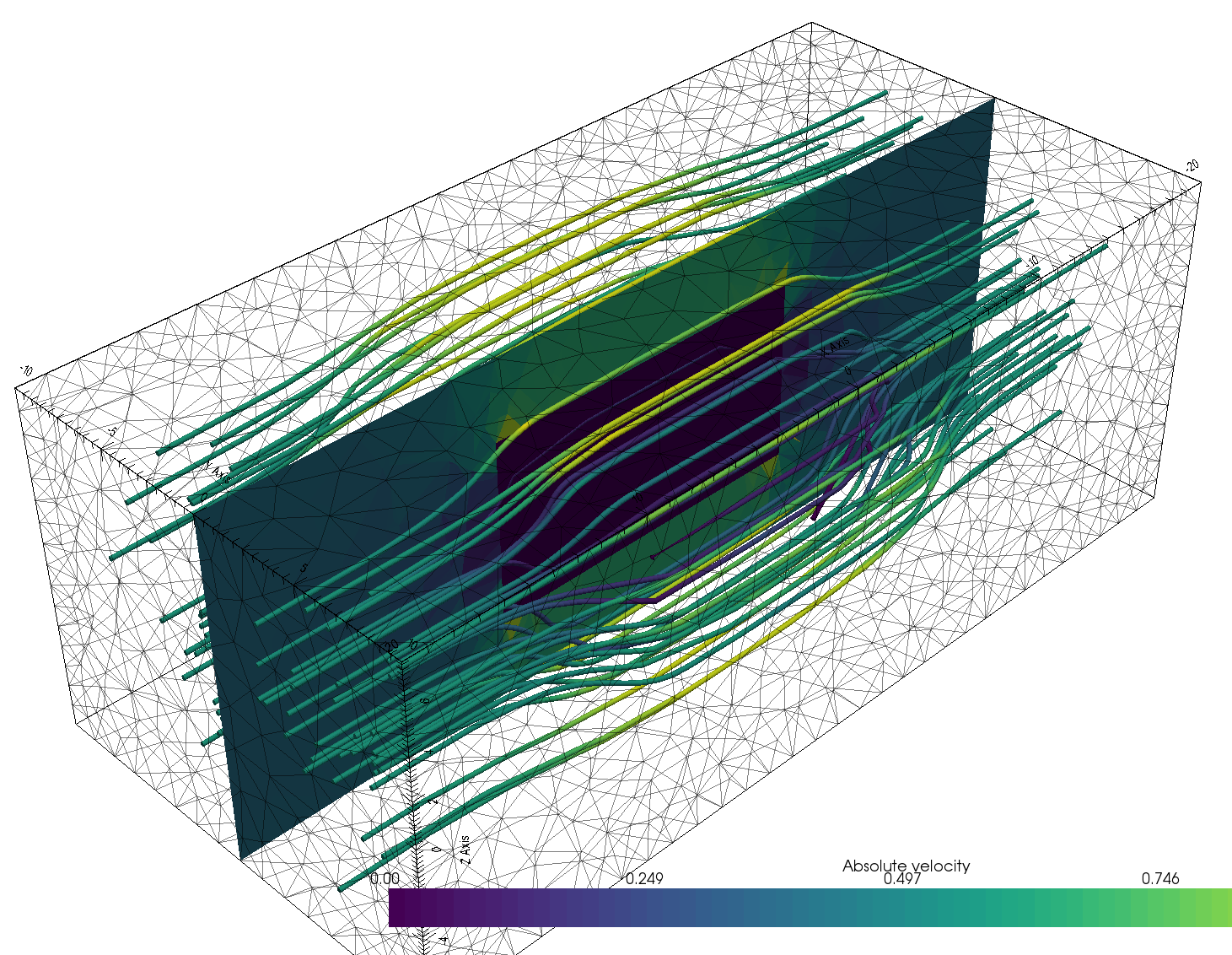
pyGIMLi is a versatile open-source toolbox with:

  • management tools for structured and unstructured meshes in 2D & 3D
  • computationally efficient finite-element and finite-volume solvers
  • various geophysical forward operators: ERT/IP, Traveltime, Gravimetry, Magnetics, SP, EM
  • frameworks for constrained, joint and process-based inversions with region-specific regularization
  • open-source, platform compatible, documented & tested code
  • suitability for teaching & reproducible research
  • v1.0 published in Computers and Geosciences (Rücker et al., 2017) (among 5 Most Downloaded papers and > 700 citations) and broadly used since
  • Website and documentation: https://pygimli.org
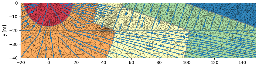
Implemented geophysical methods

All available in pygimli.physics:

Method Forward Inverse Dimension
EM ✓ ✓ 1D
ERT ✓ ✓ 2D, 3D, 4D
Gravimetry ✓ ✓ 2D, 3D
Magnetics ✓ ✓ 2D, 3D
Petrophysics ✓ ✓ dimensionless
Seismics ✓ - 2D
SIP ✓ ✓ 1D, 2D, 3D
sNMR ✓ ✓ 1D
Traveltime ✓ ✓ 2D, (3D)
VES ✓ ✓ 1D

Software design

pyGIMLi is organized in three different abstraction levels:

In the application level, ready-to-use method managers and frameworks are provided.

from pygimli.physics import ert
mgr = ert.ERTManager("mydata.dat")
mgr.showData()
mgr.invert(lam=50)
mgr.showResult()

In the modelling level, users can set up customized forward operators that map discretized parameter distributions to a data vector. Once defined, it is straightforward to set up a corresponding inversion workflow or combine the forward operator with existing ones.

rho_a = ert.simulate(mesh, scheme,model)

The underlying equation level allows to directly access the finite element solvers to solve various partial differential equations on unstructured meshes, i.e. to approach various physical problems with possibly complex 2D and 3D geometries.
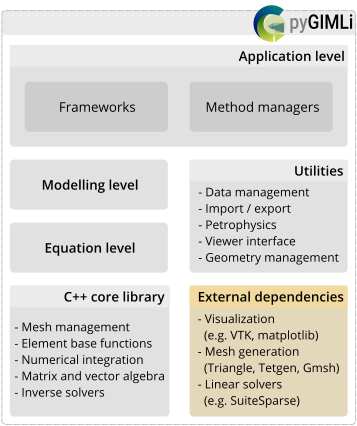
Rücker et al. (2017)

Basic inversion framework

The default inversion framework is based on the generalized Gauss-Newton method and is compatible with any given forward operator and thus applicable to various physical problems.

\[ \| \mathbf{W}_\text{d} (\mathbf{F}(\mathbf{m})-\mathbf{d}) \|^2_2 + \lambda \| \mathbf{W}_\text{m} (\mathbf{m}-\mathbf{m_0}) \|^2_2 \rightarrow\min \]

Note

The inversion is physics-independent and very flexible in terms of adding prior information, regularization and integrating different geophysical methods.
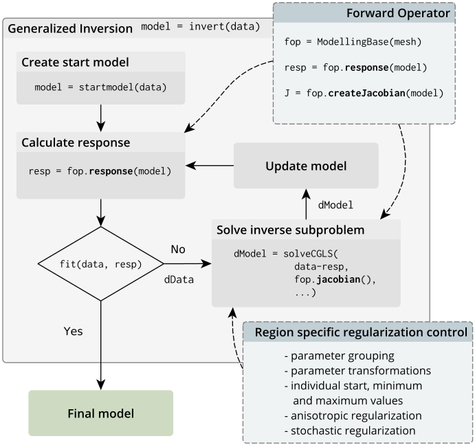
Rücker et al. (2017)

Recent developments in pyGIMLi

  • Improved 3D visualization powered by pyvista (including filters, slices and interactive notebook compatibility)
  • 3D gravity and (full-tensor) magnetics operators and managers
  • LSQRinversion framework enabling additional parameter relations (from Wagner et al., 2019)
  • MultiFrameModelling framework for temporally/spectrally/spatially constrained inversion
  • TimelapseERT class with different strategies, e.g. 4D inversion
  • New examples on ERT (2D/3D crosshole, 3D surface, timelapse), IP, 3D magnetics
  • Improved website and new user-guide
  • enabled pip install pygimli for easier installation (e.g. on Google Colab)
  • fully complex-valued (FD) ERT-IP inversion (also for TD)
  • Structurally-coupled cooperative (SCCI) inversion framework

Existing tutorials

  • Transform 2021: creating geometries & meshes, modeling PDEs, synthetic data, inversion (also with external forward operator).
  • Transform 2022: fundamental pyGIMLi objects (Mesh, DataContainer, matrix types, etc.), geostatistical vs. smoothness regularization, treatment of subsurface regions, adding prior data.
  • SEG webinar 2024: invert real-life 3D data (Hübner et al., 2017) to tweak your inversion beyond the standard practice.
  • GELMON 2025: ERT time-lapse data processing and inversion + image appraisal
  • Today we focus on combining near-surface geophysical data for joint interpretation and inversion.
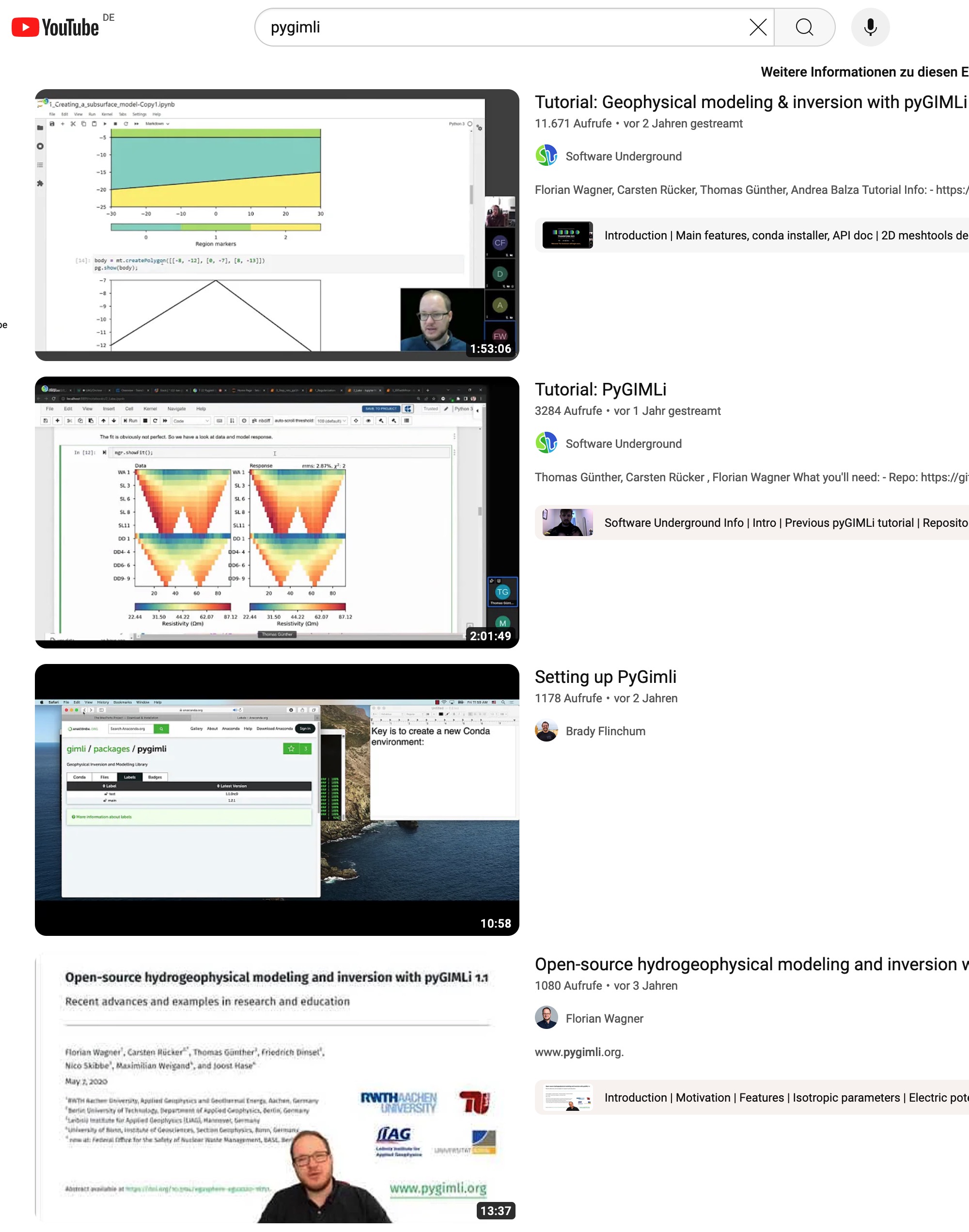
Join the pyGIMLi user community!
“In open source, we feel strongly that to really do something well, you have to get a lot of people involved.”

– Linus Torvalds

  1. Join the #pyGIMLi chat on Mattermost!
  2. Open a discussion or raise an issue on GitHub.
  3. Contribute to the website via the “Improve this page” button in the right sidebar.
  4. Add your pyGIMLi-powered publication to this database.
  5. Send your example to mail@pygimli.org.
  6. Contribute to the code as described in our contribution guidelines.

A typical ERT workflow

Everything is exposed through

import pygimli.physics.ert as ert

and the high-level ert.ERTManager class — but every step can also be customized at the modelling or equation level.

  1. Survey design — electrode geometry & measurement scheme
  2. Forward modelling — predict data from a resistivity model
  3. Loading and inspecting data — apparent-resistivity pseudosections
  4. Quality control — filter unreliable measurements
  5. Error model — weights that enter the inversion
  6. Mesh generation — discretize the parameter domain
  7. Inversion — recover the subsurface resistivity model
  8. Appraisal — coverage, data fit, sensitivity

Unified data format

pyGIMLi can read various system formats, but internally the unified data format is the basis of the DataContainer class, which is used for all data management and processing steps.

6 # Number of electrodes
# x z 
0     0
1     0
2     0 # loose ground
3     0
4     0
5     0
6 # Number of data
# a b m n u i/mA err/%
  1   2   3   4  -0.5305165 102.2 2.4
  2   3   4   5  -0.5305165 99.9  1.4
  3   4   5   6  -0.5305165 95.6  2.6
  1   2   4   5  -0.1326291 100.1 7.6
  2   3   5   6  -0.1326291 80.2 8.6 # possibly an outlier
  1   2   5   6  -0.05305165 77.3 7.5

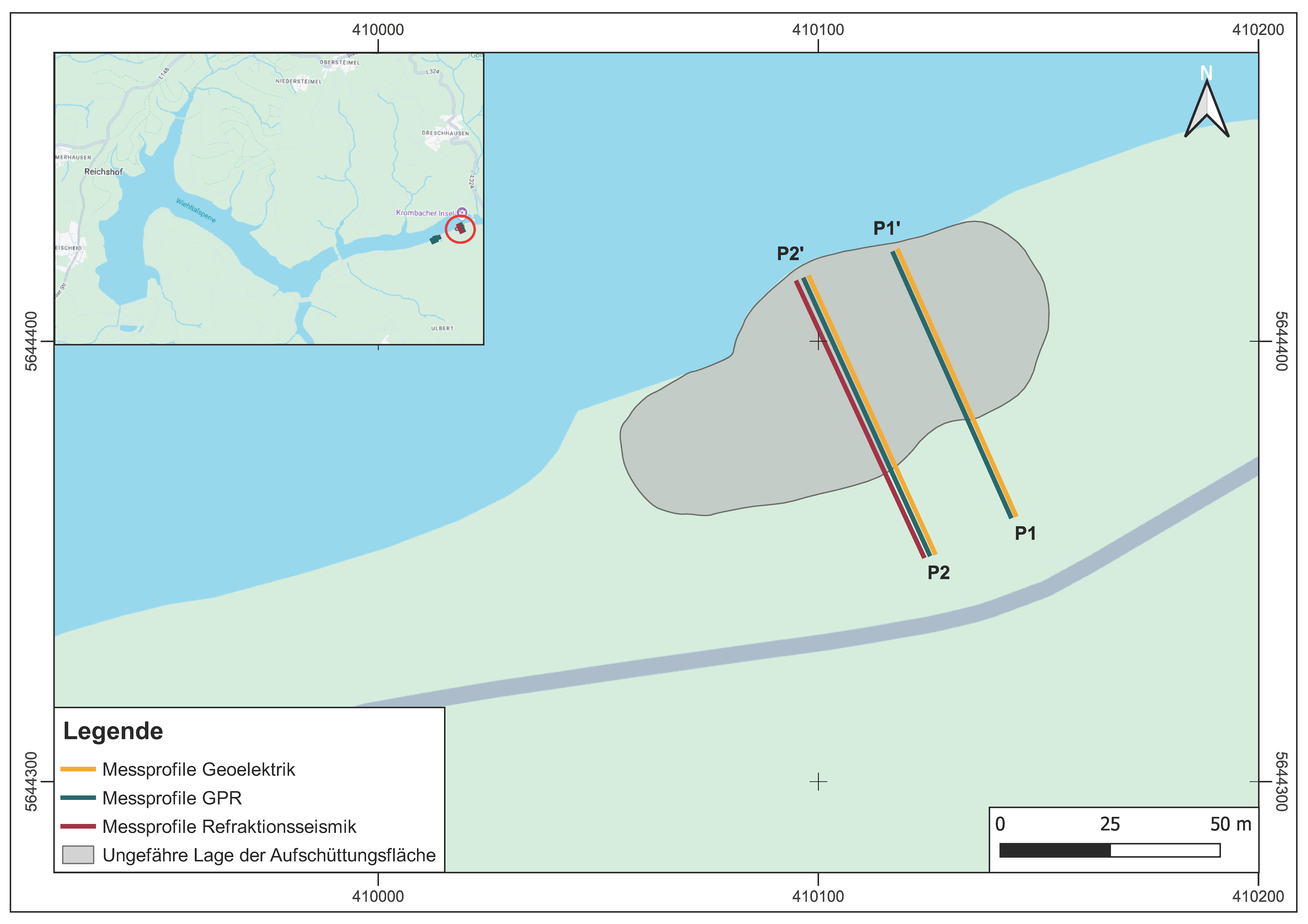
The field site - Wiehltalsperre

  • Drinking water reservoir near Cologne, Germany

  • Severe drought and beetle infestation lead to massive forest diebacks close to reservoir

  • Geophysical surveys should help to answer questions regarding hydrological settings in near-surface areas at potential reforesting sites

  • Can we use geophysics in combination with other soil parameter measurements to make suggestions regarding the reforestation of certain areas?

Quantitative imaging and monitoring is challenging
Goals of this part of the workshop

  1. Get familiar with pyGIMLI’s method managers for ERT and traveltime data.
  2. Learn basic operations such as data import, data filtering, and topography addition.
  3. Perform your first inversion using either your own field data or our provided data sets.
  4. Get to know the basic image appraisal techniques.
  5. Apply tools to compare and jointly interpret individual geophysical data sets.

Note

If you have pyGIMLi and Jupyter installed, please open an empty notebook.

Takeaway messages:

  • We familiarized ourselves with the method managers to process and invert ERT and SRT data.

  • We loaded, filtered, and inverted field data using pyGIMLi and qualitatively evaluated the results

  • We applied tools that allow us to quantitatively compare and qualitatively evaluate the single inversion results, such as…

    • 1D interpolation tools to generate synthetic geoelectrical and acoustic logs
    • data point - wise misfit examination to identify regions of decreased model goodness.
  • We implemented ways to further improve our individual inversions by penalizing individual data points with increased misfit.

Advanced inversion

Goals of this part of the workshop

  • Get to know the possibilities of including a-priori information as constraints into inversions.

  • Incorporate geological and structural a-priori information into regularization.

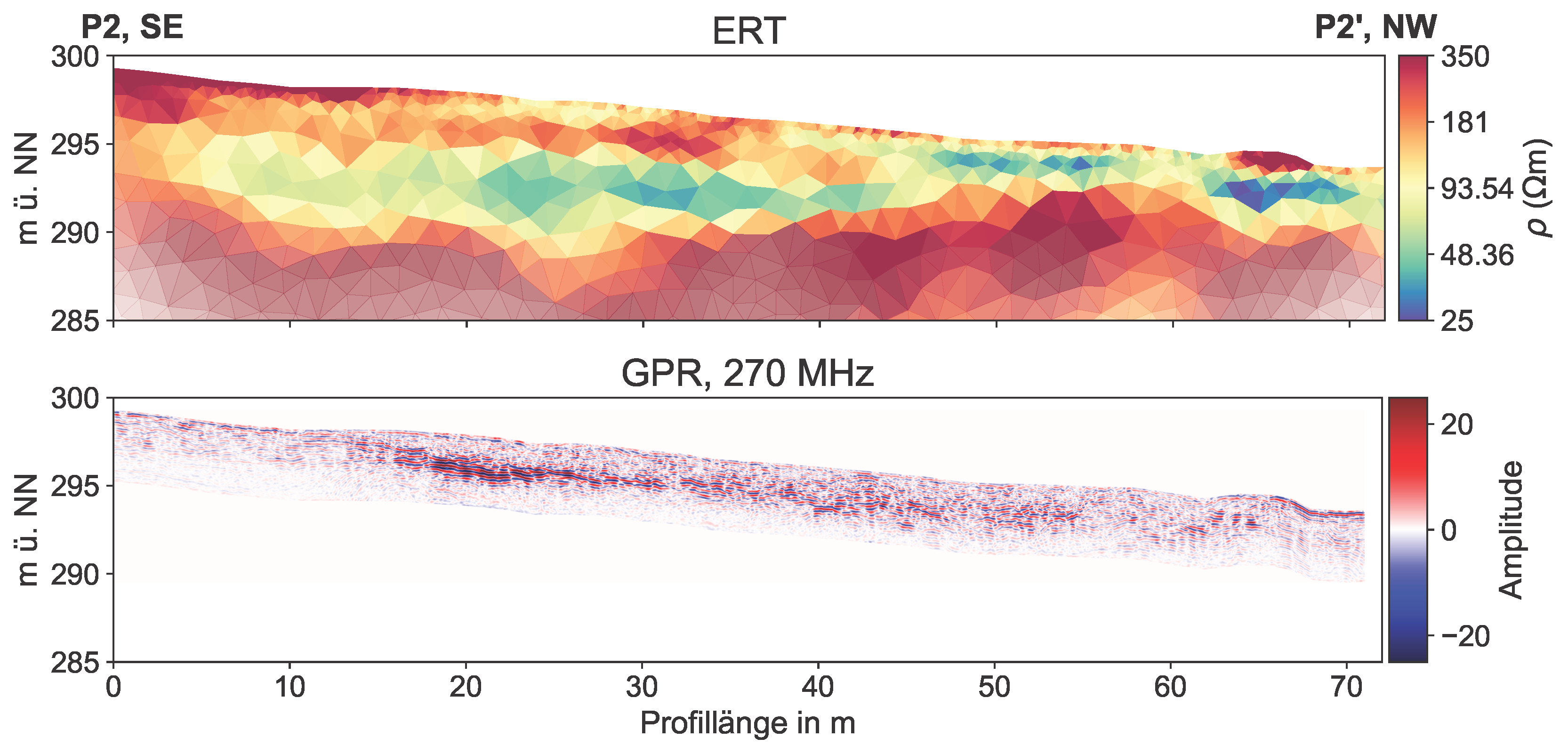
  • Incorporate reflectors visible in GPR measurements as constraints in ERT.

  • Apply interactive tools to extract constraints from images or models.

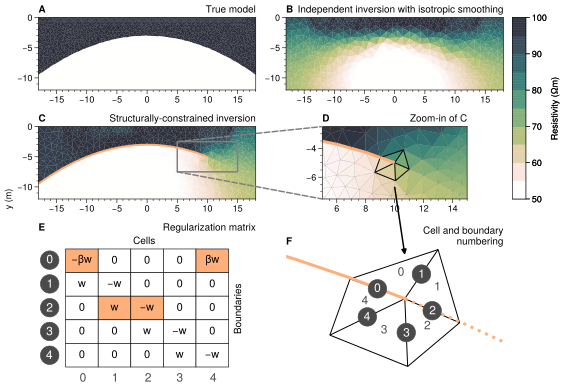
Including structural information

  • Structural information can be a useful addition to any inversion to reduce ambiguity.

  • Goal: give “hints” to the inversion as to where we expect parameter jumps / contrasts.

  • Possible sources of information:

    • wave methods (seismics, GPR,…)
    • point-wise lithological borehole information
    • geological maps or models / cross sections
    • …
  • Those information can be easily integrated into the mesh used for inversion

Implementation via smoothing matrix

Wagner & Uhlemann (2021)

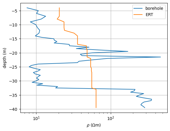
Constraints from borehole data

  • Most commonly applied constraints: including one or multiple 1D point sources of information

  • Structural / geological information or geophysical data from well logging

  • In most cases, borehole data give sharp boundaries between lithologies that can be utilized to constrain the inversion

  • Goal: by including borehole data, the inversion also aims at explaining the additional information within its error bounds, leading to an oftenmost more refined model
Geostatistical regularization

  • Alternative way to smoothness-constrained inversions using a covariance matrix to quantify the correlation of model parameters in different cells (Jordi et al., 2018)

  • Based on geological or structural analysis, an estimation of i) vertical and horizontal correlation lengths, ii) the dip angle and iii) the strike direction (in 3D) is included into the inversion

  • The resulting covariance matrix is given as:

\[ \mathbf{C}_{\text{M,i,j}} = \sigma^2 exp\left(-3 \sqrt{\left(\frac{\mathbf{H_{x,i,j}}}{I_x}\right)^2 + \left(\frac{\mathbf{H_{y,i,j}}}{I_y}\right)^2 + \left(\frac{\mathbf{H_{z,i,j}}}{I_z}\right)^2}\right) \tag{1}\]

  • Each row of the covariance matrix contains the spatial correlation function for one particular cell.

  • Example notebook: Applying geostatistical constraints

Geostatistical regularization

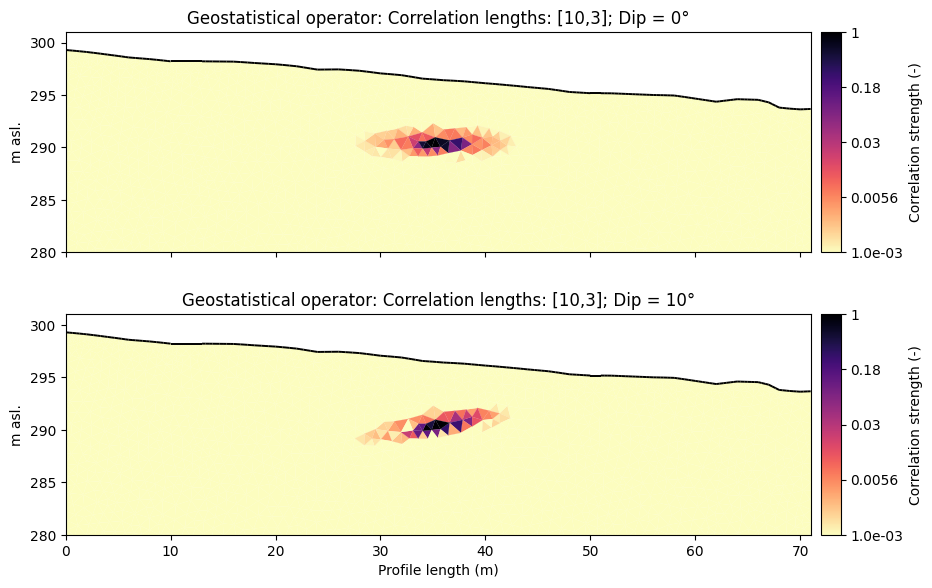
  • Alternative way to smoothness-constrained inversions using a covariance matrix to quantify the correlation of model parameters in different cells (Jordi et al., 2018)

  • Based on geological or structural analysis, an estimation of i) vertical and horizontal correlation lengths, ii) the dip angle and iii) the strike direction (in 3D) is included into the inversion

  • The resulting correlation for a single model cell looks as follows:
Inversion with two-dimensional structural constraints

  • Structural information can not only be derived from geological or structural information, but also from measurements using other geophysical methods.

  • In our case: measured GPR data are loaded and reflector is picked to define a structural constraint to further refine an ERT inversion.

  • Other possibilities: 1D downhole geophysical measurements, other wave methods (reflection seismics), …
Takeaway messages:

  • We applied advanced regularization techniques to our individual inversions

  • We constrained the individual inversions using

    • structural information on dip and geological layering
    • 1D borehole data
    • 2D GPR reflections
  • We evaluated and compared the constrained models and quantified the effect of adding a-priori information

Joint inversion

Goals of this part of the workshop

  • Learn the necessary steps to successfully perform a joint inversion.

  • Apply the cross-gradient algorithm to jointly invert SRT and ERT using actual field data.

  • Evaluate and compare the joint inversion results to individually inverted data sets.

  • Optional: Apply the algorithm to your own data sets!

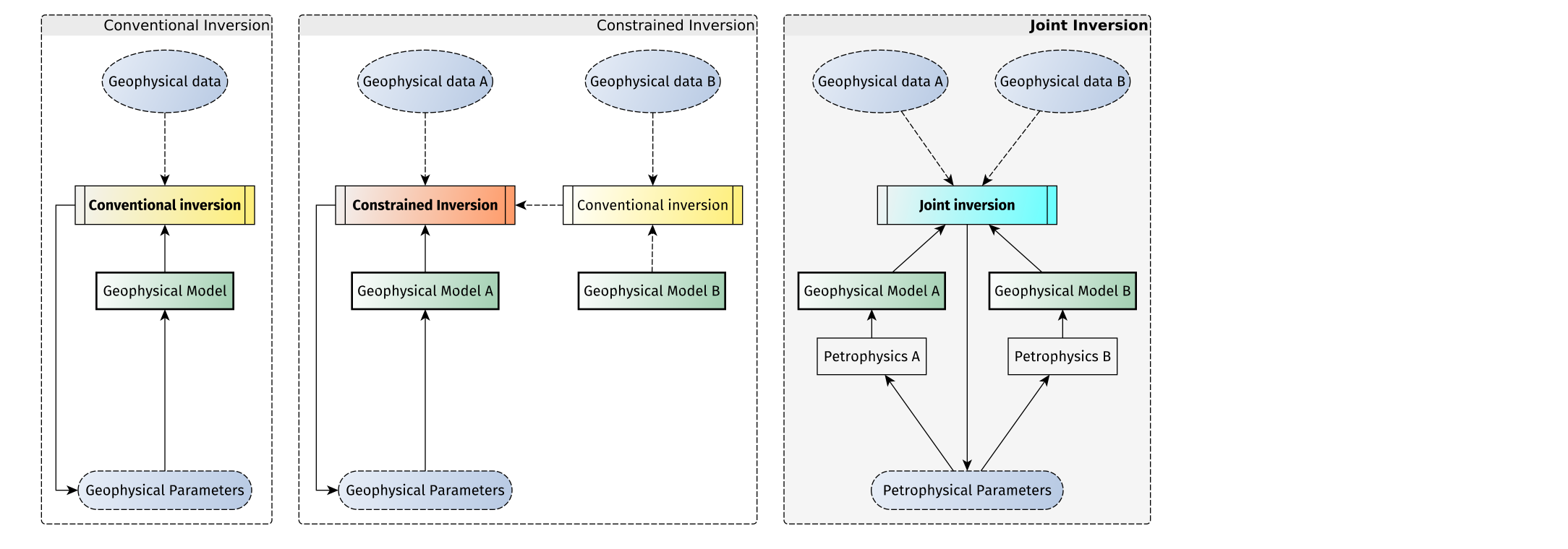
Joint inversion of methods working in same parameter space

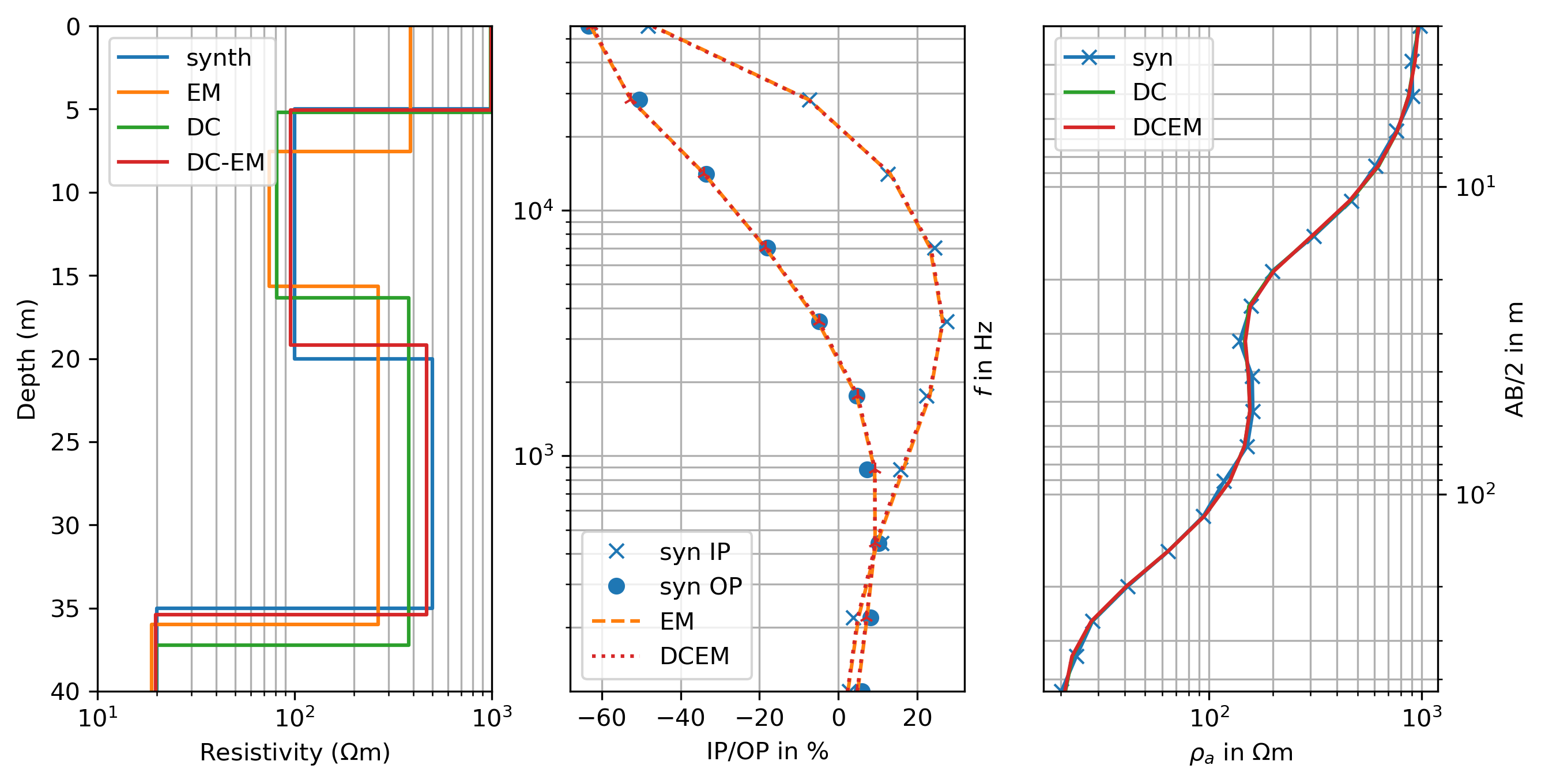
  • If two methods are sensitive to the same physical property (e.g. electrical resistivity \(\rho\) by using ERT and a electromagnetic method) we can use the same model parameter space for both methods and perform a classical joint inversion.
  • In the following example we will use vertical electrical sounding (VES) and EM data to jointly invert for the electrical resistivity distribution of the subsurface in a 1D model.
Joint inversion of methods working in different parameter spaces

Petrophysically coupled joint inversion

  • If two methods are sensitive to different physical properties (e.g. electrical resistivity \(\rho\) by using ERT and acoustic velocity \(v\) by using SRT) we can use different types of joint inversion algorithms to link the two model parameter spaces.

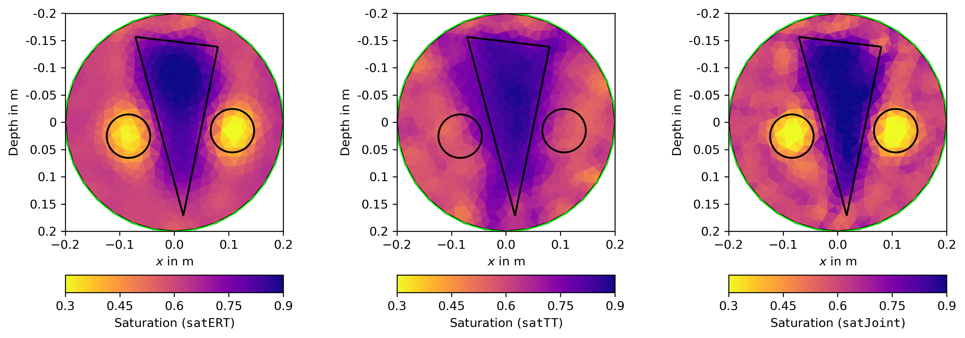
  • One possible approach is to couple both methods by using a petrophysical relationship between the two physical properties. This is called petrophysically coupled joint inversion. For example the water saturation can be used to link the electrical resistivity and acoustic velocity of the subsurface.

Joint inversion of methods working in different parameter spaces

  • Finally, we invert again in the same parameter space.

Joint inversion of methods working in different parameter spaces

Structurally coupled joint inversion

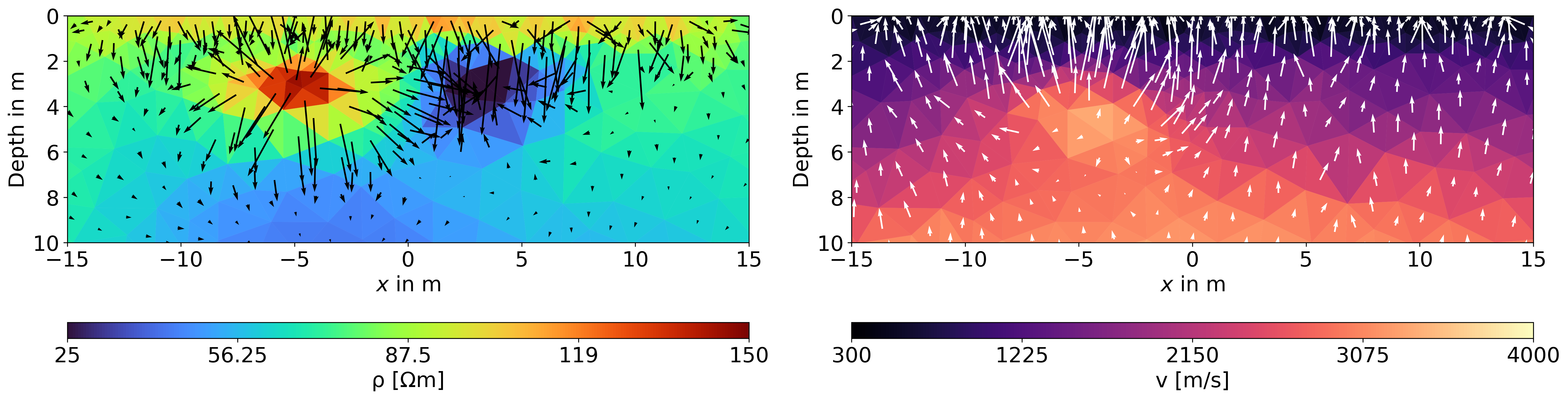
  • If a petrophysical relationship is not known or cannot be applied, we can use a structurally coupled joint inversion. In this case, we assume that the two physical properties are structurally related, i.e. they have similar spatial distributions. This can be achieved by using a cross-gradient constraint in the inversion.

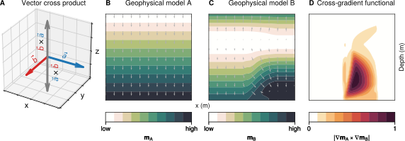
  • For this purpose, we define the cross-gradient function \(\Phi_{cg}\) as the integral of the squared magnitude of the cross product of the gradients of the two physical properties:

\[\Phi_{cg} = \int \left| \nabla \mathbf{\rho}(i) \times \nabla \mathbf{v}(i) \right|^{2}\]

The idea of cross-gradients


Wagner & Uhlemann (2021)

Joint inversion of methods working in different parameter spaces

Structurally coupled joint inversion

  • The gradients of two models in different parameter spaces are parallel if the cross-gradient function \(\Phi_{cg}\) is zero. In this case, the two models are structurally quite similar.

Takeaway messages:

  • which type of joint inversion to use depends on the physical properties of the methods used.

  • If the methods are sensitive to the same physical property, a classical joint inversion can be used.

  • If the methods are sensitive to different physical properties, a petrophysically coupled or structurally coupled joint inversion can be used.

  • A petrophysically coupled joint inversion requires a known petrophysical relationship between the two physical properties.

  • Often, a structurally coupled joint inversion is used, which requires no petrophysical relationship between the two physical properties.

References

Binley, A., Hubbard, S. S., Huisman, J. A., Revil, A., Robinson, D. A., Singha, K., & Slater, L. D. (2015). The emergence of hydrogeophysics for improved understanding of subsurface processes over multiple scales. Water Resources Research, 51(6), 3837–3866. https://doi.org/https://doi.org/10.1002/2015WR017016
Hübner, R., Günther, T., Heller, K., Noell, U., & Kleber, A. (2017). Impacts of a capillary barrier on infiltration and subsurface stormflow in layered slope deposits monitored with 3-d ERT and hydrometric measurements. Hydrology and Earth System Sciences, 21(10), 5181–5199. https://doi.org/10.5194/hess-21-5181-2017
Jordi, C., Doetsch, J., Günther, T., Schmelzbach, C., & Robertsson, J. O. A. (2018). Geostatistical regularization operators for geophysical inverse problems on irregular meshes. Geophysical Journal International, 213(2), 1374–1386. https://doi.org/10.1093/gji/ggy055
Rücker, C., Günther, T., & Wagner, F. M. (2017). pyGIMLi: An open-source library for modelling and inversion in geophysics. Computers and Geosciences, 109, 106–123. https://doi.org/10.1016/j.cageo.2017.07.011
Wagner, F. M., Mollaret, C., Günther, T., Kemna, A., & Hauck, C. (2019). Quantitative imaging of water, ice, and air in permafrost systems through petrophysical joint inversion of seismic refraction and electrical resistivity data. Geophysical Journal International, 219(3), 1866–1875. https://doi.org/10.1093/gji/ggz402
Wagner, F. M., & Uhlemann, S. (2021). An overview of multimethod imaging approaches in environmental geophysics. Advances in Geophysics, Vol. 44, 62, 1–72. https://doi.org/10.1016/bs.agph.2021.06.001